How it currently works Pt.1
In this post Id like to discuss the current setup of the program to show how I set it up and how it can be used!
Because I am also working on EMerge as a Physical Optics solver with other post processing features, the fem solver is hidden away in a submodule inside the module EMerge. In the following example we are going to make a weird filtering waveguide antenna at X-band. We are going to use the filter dimensions from a Comsol tutorial.
First we start by loading the fem module in our namespace and defining our parameters.
The setup of the simulation file.
The next step is for us to start our simulation model. The meshing is done using the open source GMSH library. This library requires you to call the gmsh.finalize() function after being done with the process. For this reason I created a simple with-statement for the model class which is mostly used to manage all the important simulation file data and thus also call GMSH’s finalize function.
The Comsol filter contains four irises which are symmetrical, last two are the first two in reverse. For that reason we will make one quarter of the waveguide and then mirror it.
The code which creates the quarter waveguide section (half length, half width) and subtracts the irises.
As you can see we start with the with statement which will return a Simulation2D object. Next we call the rectcenter() function. This function returns a Shapely Polygon object. In that sense, rect_center() is just a convenient macro that generates the Shapely Polygon. The same is true for the two irises. Next the irises are subtracted from the waveguide using the Shapely class methods directly, no EMerge involved here!
Finally, we put the waveguide in a list and give it to the model using the set_polygons method (name may change). This method will take all polygons and generate a set of fully disjoint polygons (no overlapping space). These will have uniquely numbered edges and domains. These numbers are called tags, which are used by GMSH to link the mesh nodes to the source geometry.
Our model object also contains several classes as attributes that we will learn about later. The one that is important now is the Geometry class. The geometry class manages all boundaries, edges and vertices contained in our geometry. We can see what comes out by calling the overview method on the Geometry class.
The output of the overview() method.
As we can see we have one quarter of our filter. Next we will mirror the filter twice and then look at the geometry again.
The code with the mirror statements.
The complete waveguide filter.
The mirroring operation caused quite a mess. We have 4 separate domains and lots of edges. In principle we could assign the port boundaries to 21, 32 and 9 with 42 but in this case its probably easier to just unite all the geometries using shapely and then to pass them to the polygon method. Shapely offers us this feature with the union function. We also call the simplify() method on the final geometry to effectively remove the vertex that splits the boundary into 21,32 and 9,42. Furthermore, we will use .mirror() method on the resultant geometries to save ourselves some work.
The waveguide generation with the mirroring and union.
The simpilfied waveguide filter geometry.
Next we are going to assign the two port boundary conditions. To do this we are introduced to another attribute of our model: the physics attribute. The physics attribute is a Physics class object which now only represents frequency domain physics. There will be different distinct physics classes for different types of physics such as electrostatics or heat transfer later in the development.
To assign our boundary conditions we use the appropriately named .assign() method. The first argument will be the boundary condition which in this case can be found in the bc (boundary condition) submodule. We use the Port boundary condition and number them appropriately. The active parameter defines which will radiate the energy into our domain. The second argument of our assign function is the edge keyword argument. The other keyword argument you could use is edges in case we want to assign more than one at the same time. For this we must provide an Edge object. This object can be retrieved using the select method on the Geometry class. This select method simply takes and x,y coordinate argument and returns a Selection object that contains a point, edge and domain closest to that point. In this case we can take the edge attribute to give us the Edge object we need. This edge object will contain the relevant information which in this case is the tag number corresponding to the edge at our input and output port. This way we do not have to change our numbering every time we change the geometry and the labelling.
After setting our boundary conditions we set our model resolution to 0.3 lambda (maximum mesh size in terms of the wavelength) and the frequency range. We can then call the generate_mesh() method to generate our mesh.
The code that adds boundary conditions, sets the frequency range and generates the mesh.
The generated mesh including the quadratic basis function vertices.
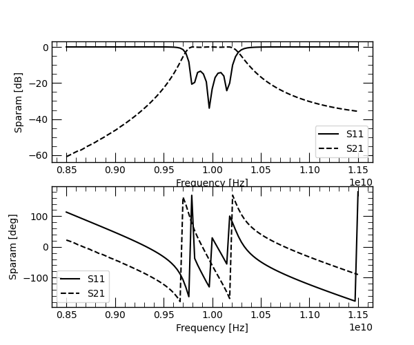
We can see the output mesh generated by GMSH. Our last step is to simply call the run frequency domain method which will return a Dataset2D object containing the relevant field data. We can use the convenient S-parameter plot function and the plot field function to see our results. The current port numbering in the plot does not correspond with the provided numbering if we were to assign different arbitrary numbers.
In the final run simulation I changed the number of frequency points to 101. For reference, that simulation took just 9 seconds. This can be reduced significantly once the matrix assembly algorithm is ported either to a Numba compiled function or using Rust. The other half of the solving is dedicated to the BiConjugate Gradient Stabilised method or BiCGStab in SciPy’s sparse submodule. Other solving algorithms may also be used such as Numpy’s solve or GMRES etc. The matrix assembly algorithm is currently just a Phython for-loop which means a lot of optimisation may still be done!
The final three lines running the simulation.
The computed S-parameters.
The field at an arbitrary index somewhere in the stop band.
Conclusion
As we can see the setting up of the simulation and running was very trivial. Its likely that this will get more complicated as new features are added as sufficient flexibility needs to be build in order to have a program that isn’t a complete spaghetti mess. One will always notice that the most versatile programs are the most complex. The simpler you set something up, the more difficult it is to add features.
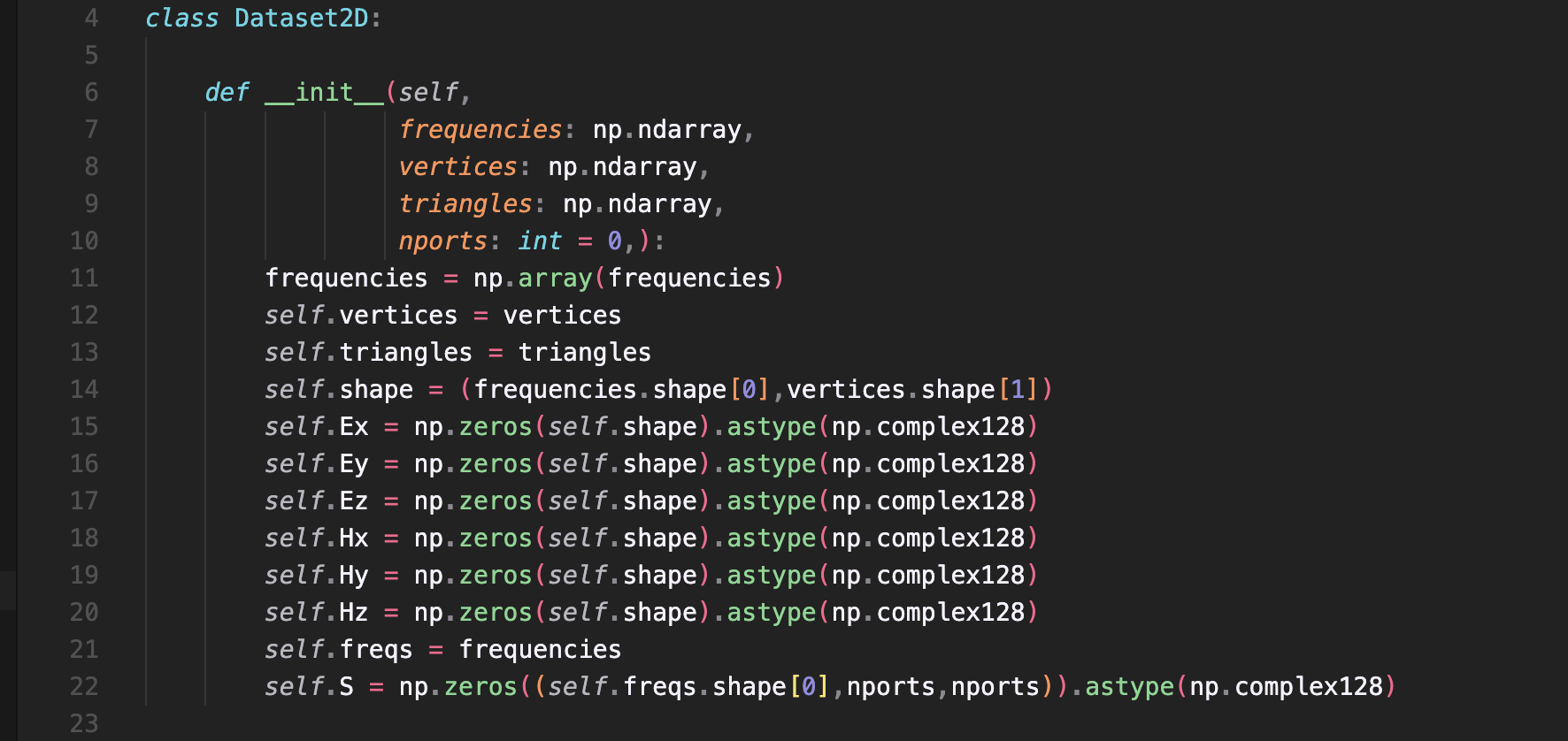
In the next section we will add a horn to the filter and implement absorbing boundaries to show this feature as well. As a closing statement I would like to demonstrate what the current implementation of the Dataset2D class is. It is, in fact very barebones. For now it is just a class that contains the typical field parameters. Naturally because this solver is only solving for the Ez-field, lots of the provided data contains just zero’s. It does however show just how accessible the resultant data is to the end user. Such a class is much easier to deal with than some strange .csv file with mesh and field data.
Note that this current implementation is not ideal by any stretch of the imagination. As mentioned, EMerge is in very early phase so this implementation, just like many others will be much neater than what it is now!
The extremely simple Dataset2D class implementation


